The overall goal of this Pageturner Project is to produce an app that recognizes musical notation in pdf files, recognizes sounds as particular notes played by particular instruments, and turns the pages of the pdf when appropriate, similar to how a human pageturner would behave. This capability could also then be used for other related tasks, such as helping to train sight-readers by showing only a block of musical notation that is always a few measures ahead of where the sight-reader is playing.

The approach will be to quickly devise a Minimum Viable Product and then refine it if / as necessary to suit demand. The overall functionality will be split into three sections for development: (1) auditory note recognition, (2) optical musical notation recognition, and (3) combining them to follow along with playing (including dealing with incorrectly played or incorrectly recognized notes).

The first step, which is described in this post, is to devise an initial system for auditory note recognition. For a start, we will consider the simple case of one note being played at a time, and then later deal with the challenge of multiple notes (but noting that the manner in which the simple case is dealt with will help in dealing with the multiple-notes case).

The source code for everything described below can be found here. The pyaudio library is used for reading in microphone audio. The numpy, scipy and sklearn libraries are used in the analysis. Two demos are included, one with matplotlib and the other with a flask.py server and d3.js.

Problem Setup and Training Data

The system's task is the following: at each timestep (e.g. 20 milliseconds), collect a short audio clip and return a string stating which note is being played (or state that no notes are being played, if that is the case).

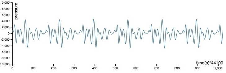
As with most standard audio recordings, the frame rate used in this case is 44100 samples / second. The audio clips sent to the system for analysis are 1024 frames in length. An example audio clip is graphed below.

Labeled training data for this test were produced using a trusty old Melodica, collecting samples of each note being played (with variable intensity) and storing them with their labels (in this case by storing them in named folders, see recorder.py in the github repo). The data set contains 14190 samples.

Machine Learning: Feature Extraction - Fourier Transformation

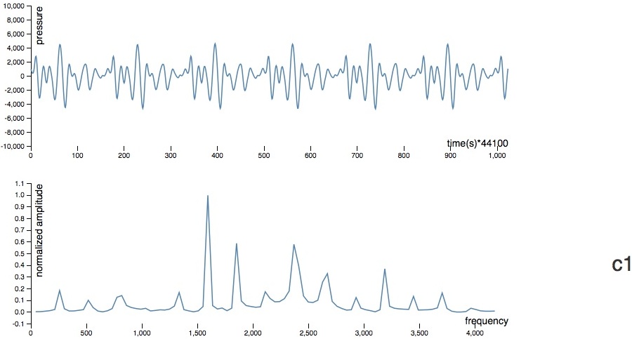
In theory, one could probably train a classifier using these sampled audio wave forms directly, but it would likely be relatively inefficient or ineffective. A more promising approach is to transform the audio waves from their given time-domain form into a frequency-domain form. The details of this Fourier Transformation are rather complicated, but the basic notion is simple in this case - we want to know the amplitudes at various frequencies in our audio sample, and the Fourier Transformation provides us with just that. Below is an example audio wave form and its frequency-amplitude equivalent.

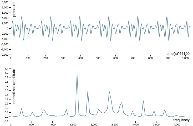
Note that, from trial and error, it turns out that normalizing the resulting amplitudes for a given sample to [0,1] makes a big difference in learning effectiveness. Also note that there may be benefits of this approach for dealing with multiple notes in unison as well, since they should be largely additive in the frequency domain.

When given one of our waveforms, the FFT (Fast Fourier Transform) algorithm outputs frequency-amplitude arrays of length 97 (note that this is after trimming them to only include frequencies within the range of notes on a piano). These arrays are used as the feature array for training and using for our machine learning system.

Machine Learning: Training and Cross-Validation - SVM

The sklearn implementation of a SVM (Support Vector Machine), with the sklearn defaults, was used to train a classifier using the transformed labeled training data set, with the training data randomly split 70%-30% into training and validation sets. (See training.py and perfectpitch.py ('train' method) in the github repo for details.) The SVM performs very well on the training set, with a training accuracy of 99.5% and a validation accuracy of 99.4%. The training process requires less than a minute on my mac air. The pickled SVM is persisted in a 15.1 MB text file.

Watching it in Action

The screencaptures below show the demo web app in action. It performs surprisingly well for a first pass. Occasionally it misclassifies a note (most often confusing a note as being an octave higher or lower, e.g. a C1 instead of a C2, which makes sense because of resonant frequencies), and it sometimes confuses the sound of speech for the sound of a note - both of these challenges can probably be easily overcome by adding more varied training data.

Next Steps

This first step will certainly be revisited again in order to deal with multiple notes in unison, and also to improve performance. But as it stands it works well enough to use as a starting point. As such, the next step will be to devise an optical musical notation recognition system (or select an existing one for adoption and integration).